What are Diffusion Models?

Introduction: Generative Models

Given observed samples $\boldsymbol{x}$ from a distribution of interest, the goal of the generative model is to learn to model its true data distribution $p(\boldsymbol{x})$ . Once learned, we can generate new samples from our approximate model at will. Furthermore, under some formulations, we are able to use the learned model to evaluate the likelihood of observed or sampled data as well.

Background: ELBO, VAE, and Hierarchical VAE

Evidence Lower Bound
Mathematically, we can imagine the latent variables and the data we observe as modeled by a joint distribution $p(\boldsymbol{x}, \boldsymbol{z})$ . Recall one approach of generative modeling, termed “likelihood-based”, is to learn a model to maximize the likelihood $p(\boldsymbol{x})$ of all observed $\boldsymbol{x}$ . There are two ways we can manipulate this joint distribution to recover the likelihood of purely our observed data $p(\boldsymbol{x})$ ; we can explicitly marginalize out the latent variable $\boldsymbol{z}$ .

$\centering p(\boldsymbol{x})=\int p(\boldsymbol{x}, \boldsymbol{z}) d \boldsymbol{z}$

Denote $q_\phi(\boldsymbol{z} \mid \boldsymbol{x})$ is a flexible approximate variational distribution with parameters $\boldsymbol{\phi}$ that we seek to optimize.

$\begin{aligned} \log p(\boldsymbol{x}) & =\log p(\boldsymbol{x}) \int q_{\boldsymbol{\phi}}(\boldsymbol{z} \mid \boldsymbol{x}) d z \\ & =\int q_{\boldsymbol{\phi}}(\boldsymbol{z} \mid \boldsymbol{x})(\log p(\boldsymbol{x})) d z \\ & =\mathbb{E}_{q_\phi(\boldsymbol{z} \mid \boldsymbol{x})}[\log p(\boldsymbol{x})] \\ & =\mathbb{E}_{q_\phi(\boldsymbol{z} \mid \boldsymbol{x})}\left[\log \frac{p(\boldsymbol{x}, \boldsymbol{z})}{p(\boldsymbol{z} \mid \boldsymbol{x})}\right] \\ & =\mathbb{E}_{q_\phi(\boldsymbol{z} \mid \boldsymbol{x})}\left[\log \frac{p(\boldsymbol{x}, \boldsymbol{z}) q_\phi(\boldsymbol{z} \mid \boldsymbol{x})}{p(\boldsymbol{z} \mid \boldsymbol{x}) q_\phi(\boldsymbol{z} \mid \boldsymbol{x})}\right] \\ & =\mathbb{E}_{q_\phi(\boldsymbol{z} \mid \boldsymbol{x})}\left[\log \frac{p(\boldsymbol{x}, \boldsymbol{z})}{q_\phi(\boldsymbol{z} \mid \boldsymbol{x})}\right]+\mathbb{E}_{q_\phi(\boldsymbol{z} \mid \boldsymbol{x})}\left[\log \frac{q_\phi(\boldsymbol{z} \mid \boldsymbol{x})}{p(\boldsymbol{z} \mid \boldsymbol{x})}\right] \\ & =\mathbb{E}_{q_\phi(\boldsymbol{z} \mid \boldsymbol{x})}\left[\log \frac{p(\boldsymbol{x}, \boldsymbol{z})}{q_{\boldsymbol{\phi}}(\boldsymbol{z} \mid \boldsymbol{x})}\right]+D_{\mathrm{KL}}\left(q_\phi(\boldsymbol{z} \mid \boldsymbol{x}) \| p(\boldsymbol{z} \mid \boldsymbol{x})\right) \\ & \geq \mathbb{E}_{q_\phi(\boldsymbol{z} \mid \boldsymbol{x})}\left[\log \frac{p(\boldsymbol{x}, \boldsymbol{z})}{q_{\boldsymbol{\phi}}(\boldsymbol{z} \mid \boldsymbol{x})}\right] \end{aligned}$

From this derivation, we clearly observe that the evidence is equal to the ELBO plus the KL Divergence between the approximate posterior $q_\phi(\boldsymbol{z} \mid \boldsymbol{x})$ and the true posterior $p(\boldsymbol{z} \mid \boldsymbol{x})$ .

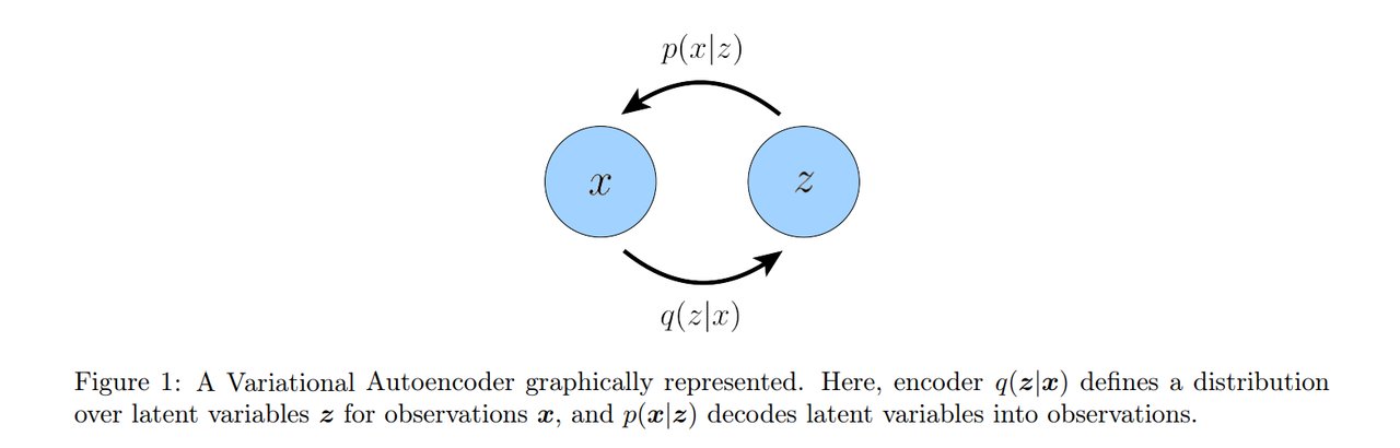
Variational Autoencoders
In the default formulation of the Variational Autoencoder (VAE), we directly maximize the ELBO. This approach is variational, because we optimize for the best $q_\phi(\boldsymbol{z} \mid \boldsymbol{x})$ amongst a family of potential posterior distributions parameterized by $\phi$ .

$\begin{aligned} & \mathbb{E}_{q_{\boldsymbol{\phi}}(\boldsymbol{z} \mid \boldsymbol{x})}\left[\log \frac{p(\boldsymbol{x}, \boldsymbol{z})}{q_{\boldsymbol{\phi}}(\boldsymbol{z} \mid \boldsymbol{x})}\right]=\mathbb{E}_{q_{\boldsymbol{\phi}}(\boldsymbol{z} \mid \boldsymbol{x})}\left[\log \frac{p_{\boldsymbol{\theta}}(\boldsymbol{x} \mid \boldsymbol{z}) p(\boldsymbol{z})}{q_{\boldsymbol{\phi}}(\boldsymbol{z} \mid \boldsymbol{x})}\right] \\ & =\mathbb{E}_{q_\phi(\boldsymbol{z} \mid \boldsymbol{x})}\left[\log p_{\boldsymbol{\theta}}(\boldsymbol{x} \mid \boldsymbol{z})\right]+\mathbb{E}_{q_{\boldsymbol{\phi}}(\boldsymbol{z} \mid \boldsymbol{x})}\left[\log \frac{p(\boldsymbol{z})}{q_{\boldsymbol{\phi}}(\boldsymbol{z} \mid \boldsymbol{x})}\right] \\ & =\underbrace{\mathbb{E}_{q_{\boldsymbol{\phi}}(\boldsymbol{z} \mid \boldsymbol{x})}\left[\log p_{\boldsymbol{\theta}}(\boldsymbol{x} \mid \boldsymbol{z})\right]}_{\text {reconstruction term }}-\underbrace{D_{\mathrm{KL}}\left(q_{\boldsymbol{\phi}}(\boldsymbol{z} \mid \boldsymbol{x}) \| p(\boldsymbol{z})\right)}_{\text {prior matching term }} \\ & \end{aligned}$

In this case, we learn an intermediate bottlenecking distribution $q_\phi(\boldsymbol{z} \mid \boldsymbol{x})$ that can be treated as an encoder; it transforms inputs into a distribution over possible latents. Simultaneously, we learn a deterministic function $p_{\boldsymbol{\theta}}(\boldsymbol{x} \mid \boldsymbol{z})$ to convert a given latent vector $\boldsymbol{z}$ into an observation $\boldsymbol{x}$ , which can be interpreted as a decoder.

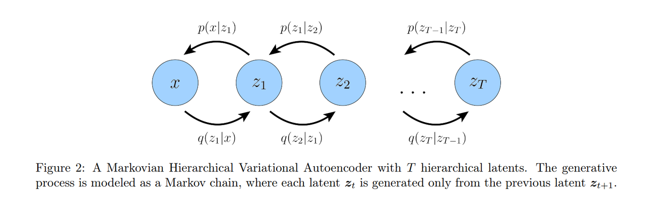
Hierarchical Variational Autoencoders

A Hierarchical Variational Autoencoder (HVAE) is a generalization of a VAE that extends to multiple hierarchies over latent variables. Under this formulation, latent variables themselves are interpreted as generated from other higher-level, more abstract latents.
Whereas in the general HVAE with T hierarchical levels, each latent is allowed to condition on all previous latents, in this work we focus on a special case which we call a Markovian HVAE (MHVAE). In a MHVAE, the generative process is a Markov chain; that is, each transition down the hierarchy is Markovian, where decoding each latent $\boldsymbol{z}_t$ only conditions on previous latent $\boldsymbol{z}_{t+1}$ .
Intuitively, and visually, this can be seen as simply stacking VAEs on top of each other, as depicted in Figure 2; another appropriate term describing this model is a Recursive VAE. Mathematically, we represent the joint distribution and the posterior of a Markovian HVAE as:

$\begin{aligned} p\left(\boldsymbol{x}, \boldsymbol{z}_{1: T}\right) & =p\left(\boldsymbol{z}_T\right) p_{\boldsymbol{\theta}}\left(\boldsymbol{x} \mid \boldsymbol{z}_1\right) \prod_{t=2}^T p_{\boldsymbol{\theta}}\left(\boldsymbol{z}_{t-1} \mid \boldsymbol{z}_t\right) \\ q_{\boldsymbol{\phi}}\left(\boldsymbol{z}_{1: T} \mid \boldsymbol{x}\right) & =q_{\boldsymbol{\phi}}\left(\boldsymbol{z}_1 \mid \boldsymbol{x}\right) \prod_{t=2}^T q_{\boldsymbol{\phi}}\left(\boldsymbol{z}_t \mid \boldsymbol{z}_{t-1}\right) \end{aligned}$

Then, we can easily extend the ELBO to be:

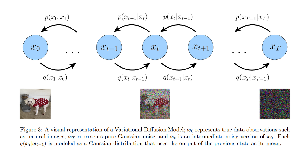
$\begin{aligned} \log p(\boldsymbol{x}) & =\log \int p\left(\boldsymbol{x}, \boldsymbol{z}_{1: T}\right) d \boldsymbol{z}_{1: T} \\ & =\log \int \frac{p\left(\boldsymbol{x}, \boldsymbol{z}_{1: T}\right) q_{\boldsymbol{\phi}}\left(\boldsymbol{z}_{1: T} \mid \boldsymbol{x}\right)}{q_{\boldsymbol{\phi}}\left(\boldsymbol{z}_{1: T} \mid \boldsymbol{x}\right)} d \boldsymbol{z}_{1: T} \\ & =\log \mathbb{E}_{q_{\boldsymbol{\phi}}\left(\boldsymbol{z}_{1: T} \mid \boldsymbol{x}\right)}\left[\frac{p\left(\boldsymbol{x}, \boldsymbol{z}_{1: T}\right)}{q_{\boldsymbol{\phi}}\left(\boldsymbol{z}_{1: T} \mid \boldsymbol{x}\right)}\right] \\ & \geq \mathbb{E}_{q_{\boldsymbol{\phi}}\left(\boldsymbol{z}_{1: T} \mid \boldsymbol{x}\right)}\left[\log \frac{p\left(\boldsymbol{x}, \boldsymbol{z}_{1: T}\right)}{q_{\boldsymbol{\phi}}\left(\boldsymbol{z}_{1: T} \mid \boldsymbol{x}\right)}\right] \end{aligned}$

Variational Diffusion Models

The easiest way to think of a Variational Diffusion Model (VDM is simply as a Markovian Hierarchical Variational Autoencoder with three key restrictions:

The latent dimension is exactly equal to the data dimension.
The structure of the latent encoder at each timestep is not learned; it is pre-defined as a linear Gaussian model. In other words, it is a Gaussian distribution centered around the output of the previous timestep.
The Gaussian parameters of the latent encoders vary over time in such a way that the distribution of the latent at final timestep T is a standard Gaussian.

The VDM posterior is the same as the MHVAE posterior, but can now be rewritten as:
$\centering q\left(\boldsymbol{x}_{1: T} \mid \boldsymbol{x}_0\right)=\prod_{t=1}^T q\left(\boldsymbol{x}_t \mid \boldsymbol{x}_{t-1}\right)$

From the second assumption, we know that the distribution of each latent variable in the encoder is a Gaussian centered around its previous hierarchical latent. Unlike a Markovian HVAE, the structure of the encoder at each timestep t is not learned; it is fixed as a linear Gaussian model. We parameterize the Gaussian encoder with mean $\boldsymbol{\mu}_t\left(\boldsymbol{x}_t\right)=\sqrt{\alpha_t} \boldsymbol{x}_{t-1}$ and variance $\boldsymbol{\Sigma}_t(\boldsymbol{x}_t) = (1 - \alpha_t)\mathbf{I}$ , where the form of the coefficients are chosen such that the variance of the latent variables stay at a similar scale; in other words, the encoding process is variance-preserving. Mathematically, encoder transitions are denoted as:
$q(\boldsymbol{x}_t \mid \boldsymbol{x}_{t-1}) = \mathcal{N}(\boldsymbol{x}_t;\sqrt{\alpha}_t\boldsymbol{x}_{t-1}, (1-\alpha_t)\mathbf{I})$

The joint distribution for a VDM as:

$p(\boldsymbol{x}_{0:T}) = p(\boldsymbol{x}_T)\prod_{t=1}^Tp_{\theta}(\boldsymbol{x}_{t-1} \mid \boldsymbol{x}_t)$
where $p(\boldsymbol{x}_T) = \mathcal{N}(\boldsymbol{x}_T, \mathbf{0}, \mathbf{I})$

Like any HVAE, the VDM can be optimized by maximizing the ELBO, which can be derived as:
$\begin{aligned} & \log p(\boldsymbol{x})=\log \int p\left(\boldsymbol{x}_{0: T}\right) d \boldsymbol{x}_{1: T} \\ & =\log \int \frac{p\left(\boldsymbol{x}_{0: T}\right) q\left(\boldsymbol{x}_{1: T} \mid \boldsymbol{x}_0\right)}{q\left(\boldsymbol{x}_{1: T} \mid \boldsymbol{x}_0\right)} d \boldsymbol{x}_{1: T} \\ & =\log \mathbb{E}_{q\left(\boldsymbol{x}_{1: T} \mid \boldsymbol{x}_0\right)}\left[\frac{p\left(\boldsymbol{x}_{0: T}\right)}{q\left(\boldsymbol{x}_{1: T} \mid \boldsymbol{x}_0\right)}\right] \\ & \geq \mathbb{E}_{q\left(\boldsymbol{x}_{1: T} \mid \boldsymbol{x}_0\right)}\left[\log \frac{p\left(\boldsymbol{x}_{0: T}\right)}{q\left(\boldsymbol{x}_{1: T} \mid \boldsymbol{x}_0\right)}\right] \\ & =\mathbb{E}_{q\left(\boldsymbol{x}_{1: T} \mid \boldsymbol{x}_0\right)}\left[\log \frac{p\left(\boldsymbol{x}_T\right) \prod_{t=1}^T p_{\boldsymbol{\theta}}\left(\boldsymbol{x}_{t-1} \mid \boldsymbol{x}_t\right)}{\prod_{t=1}^T q\left(\boldsymbol{x}_t \mid \boldsymbol{x}_{t-1}\right)}\right] \\ & =\mathbb{E}_{q\left(\boldsymbol{x}_{1: T} \mid \boldsymbol{x}_0\right)}\left[\log \frac{p\left(\boldsymbol{x}_T\right) p_{\boldsymbol{\theta}}\left(\boldsymbol{x}_0 \mid \boldsymbol{x}_1\right) \prod_{t=2}^T p_{\boldsymbol{\theta}}\left(\boldsymbol{x}_{t-1} \mid \boldsymbol{x}_t\right)}{q\left(\boldsymbol{x}_T \mid \boldsymbol{x}_{T-1}\right) \prod_{t=1}^{T-1} q\left(\boldsymbol{x}_t \mid \boldsymbol{x}_{t-1}\right)}\right] \\ & =\mathbb{E}_{q\left(\boldsymbol{x}_{1: T} \mid \boldsymbol{x}_0\right)}\left[\log \frac{p\left(\boldsymbol{x}_T\right) p_{\boldsymbol{\theta}}\left(\boldsymbol{x}_0 \mid \boldsymbol{x}_1\right) \prod_{t=1}^{T-1} p_{\boldsymbol{\theta}}\left(\boldsymbol{x}_t \mid \boldsymbol{x}_{t+1}\right)}{q\left(\boldsymbol{x}_T \mid \boldsymbol{x}_{T-1}\right) \prod_{t=1}^{T-1} q\left(\boldsymbol{x}_t \mid \boldsymbol{x}_{t-1}\right)}\right] \\ & =\mathbb{E}_{q\left(\boldsymbol{x}_{1: T} \mid \boldsymbol{x}_0\right)}\left[\log \frac{p\left(\boldsymbol{x}_T\right) p_{\boldsymbol{\theta}}\left(\boldsymbol{x}_0 \mid \boldsymbol{x}_1\right)}{q\left(\boldsymbol{x}_T \mid \boldsymbol{x}_{T-1}\right)}\right]+\mathbb{E}_{q\left(\boldsymbol{x}_{1: T} \mid \boldsymbol{x}_0\right)}\left[\log \prod_{t=1}^{T-1} \frac{p_{\boldsymbol{\theta}}\left(\boldsymbol{x}_t \mid \boldsymbol{x}_{t+1}\right)}{q\left(\boldsymbol{x}_t \mid \boldsymbol{x}_{t-1}\right)}\right] \\ & =\mathbb{E}_{q\left(\boldsymbol{x}_{1: T} \mid \boldsymbol{x}_0\right)}\left[\log p_{\boldsymbol{\theta}}\left(\boldsymbol{x}_0 \mid \boldsymbol{x}_1\right)\right]+\mathbb{E}_{q\left(\boldsymbol{x}_{1: T} \mid \boldsymbol{x}_0\right)}\left[\log \frac{p\left(\boldsymbol{x}_T\right)}{q\left(\boldsymbol{x}_T \mid \boldsymbol{x}_{T-1}\right)}\right]+\mathbb{E}_{q\left(\boldsymbol{x}_{1: T} \mid \boldsymbol{x}_0\right)}\left[\sum_{t=1}^{T-1} \log \frac{p_{\boldsymbol{\theta}}\left(\boldsymbol{x}_t \mid \boldsymbol{x}_{t+1}\right)}{q\left(\boldsymbol{x}_t \mid \boldsymbol{x}_{t-1}\right)}\right] \\ & =\mathbb{E}_{q\left(\boldsymbol{x}_{1: T} \mid \boldsymbol{x}_0\right)}\left[\log p_{\boldsymbol{\theta}}\left(\boldsymbol{x}_0 \mid \boldsymbol{x}_1\right)\right]+\mathbb{E}_{q\left(\boldsymbol{x}_{1: T} \mid \boldsymbol{x}_0\right)}\left[\log \frac{p\left(\boldsymbol{x}_T\right)}{q\left(\boldsymbol{x}_T \mid \boldsymbol{x}_{T-1}\right)}\right]+\sum_{t=1}^{T-1} \mathbb{E}_{q\left(\boldsymbol{x}_{1: T} \mid \boldsymbol{x}_0\right)}\left[\log \frac{p_{\boldsymbol{\theta}}\left(\boldsymbol{x}_t \mid \boldsymbol{x}_{t+1}\right)}{q\left(\boldsymbol{x}_t \mid \boldsymbol{x}_{t-1}\right)}\right] \\ & =\mathbb{E}_{q\left(\boldsymbol{x}_1 \mid \boldsymbol{x}_0\right)}\left[\log p_{\boldsymbol{\theta}}\left(\boldsymbol{x}_0 \mid \boldsymbol{x}_1\right)\right]+\mathbb{E}_{q\left(\boldsymbol{x}_{T-1}, \boldsymbol{x}_T \mid \boldsymbol{x}_0\right)}\left[\log \frac{p\left(\boldsymbol{x}_T\right)}{q\left(\boldsymbol{x}_T \mid \boldsymbol{x}_{T-1}\right)}\right]+\sum_{t=1}^{T-1} \mathbb{E}_{q\left(\boldsymbol{x}_{t-1}, \boldsymbol{x}_t, \boldsymbol{x}_{t+1} \mid \boldsymbol{x}_0\right)}\left[\log \frac{p_{\boldsymbol{\theta}}\left(\boldsymbol{x}_t \mid \boldsymbol{x}_{t+1}\right)}{q\left(\boldsymbol{x}_t \mid \boldsymbol{x}_{t-1}\right)}\right] \\ & =\underbrace{\mathbb{E}_{q\left(\boldsymbol{x}_1 \mid \boldsymbol{x}_0\right)}\left[\log p_\theta\left(\boldsymbol{x}_0 \mid \boldsymbol{x}_1\right)\right]}_{\text {reconstruction term }}-\underbrace{\mathbb{E}_{q\left(\boldsymbol{x}_{T-1} \mid \boldsymbol{x}_0\right)}\left[D_{\mathrm{KL}}\left(q\left(\boldsymbol{x}_T \mid \boldsymbol{x}_{T-1}\right) \| p\left(\boldsymbol{x}_T\right)\right)\right]}_{\text {prior matching term }} \\ & -\sum_{t=1}^{T-1} \underbrace{\mathbb{E}_{q\left(\boldsymbol{x}_{t-1}, \boldsymbol{x}_{t+1} \mid \boldsymbol{x}_0\right)}\left[D_{\mathrm{KL}}\left(q\left(\boldsymbol{x}_t \mid \boldsymbol{x}_{t-1}\right) \| p_\theta\left(\boldsymbol{x}_t \mid \boldsymbol{x}_{t+1}\right)\right)\right]}_{\text {consistency term }} \\ & \end{aligned}$

The derived form of the ELBO can be interpreted in terms of its individual components:

$\mathbb{E}_{q\left(\boldsymbol{x}_1 \mid \boldsymbol{x}_0\right)}\left[\log p_\theta\left(\boldsymbol{x}_0 \mid \boldsymbol{x}_1\right)\right]$ can be interpreted as a reconstruction term, predicting the log probability of the original data sample given the first-step latent. This term also appears in a vanilla VAE, and can be trained similarly.
$\mathbb{E}_{q\left(\boldsymbol{x}_{T-1} \mid \boldsymbol{x}_0\right)}\left[D_{\mathrm{KL}}\left(q\left(\boldsymbol{x}_T \mid \boldsymbol{x}_{T-1}\right) \| p\left(\boldsymbol{x}_T\right)\right)\right]$ is a prior matching term; it is minimized when the final latent distribution matches the Gaussian prior. This term requires no optimization, as it has no trainable parameters; furthermore, as we have assumed a large enough T such that the final distribution is Gaussian, this term effectively becomes zero.
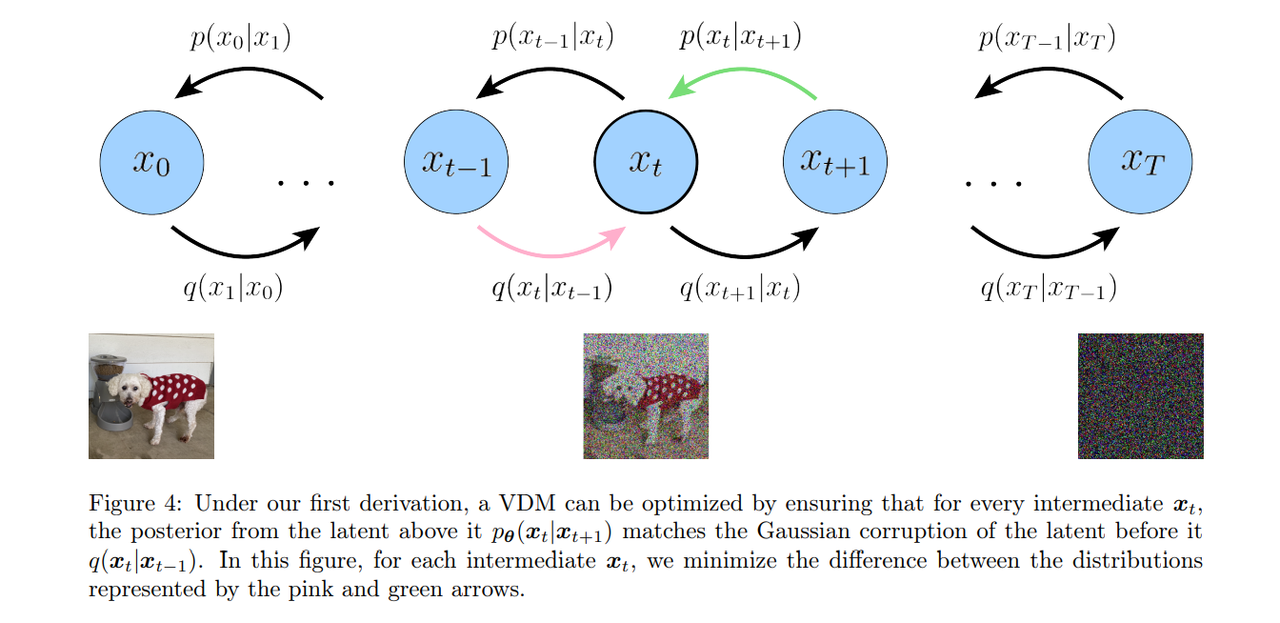
$\mathbb{E}_{q\left(\boldsymbol{x}_{t-1}, \boldsymbol{x}_{t+1} \mid \boldsymbol{x}_0\right)}\left[D_{\mathrm{KL}}\left(q\left(\boldsymbol{x}_t \mid \boldsymbol{x}_{t-1}\right) \| p_\theta\left(\boldsymbol{x}_t \mid \boldsymbol{x}_{t+1}\right)\right)\right]$ is a consistency term; it endeavors to make the distribution at $\boldsymbol{x}_t$ consistent, from both forward and backward processes. That is, a denoising step from a noisier image should match the corresponding noising step from a cleaner image, for every intermediate timestep; this is reflected mathematically by the KL Divergence. This term is minimized when we train $p_{\theta}(\boldsymbol{x}_t \mid \boldsymbol{x}_{t+1})$ to match the Gaussian distribution $q(\boldsymbol{x}_t \mid \boldsymbol{x}_{t-1})$ .

We can rewrite encoder transitions as $q(\boldsymbol{x}_t \mid \boldsymbol{x}_{t-1}) = q(\boldsymbol{x}_t \mid \boldsymbol{x}_{t-1}, \boldsymbol{x}_0)$ . Then, according to Bayes rule, we can rewrite each transition as:

$q(\boldsymbol{x}_t \mid \boldsymbol{x}_{t-1}, \boldsymbol{x}_0) = \dfrac{q(\boldsymbol{x}_{t-1} \mid \boldsymbol{x}_{t}, \boldsymbol{x}_0)q(\boldsymbol{x}_t \mid \boldsymbol{x}_0)}{q(\boldsymbol{x}_{t-1} \mid \boldsymbol{x}_0)}$

Armed with this new equation, we can retry the derivation resuming from the ELBO:

$\begin{aligned} & \log p(\boldsymbol{x}) \geq \mathbb{E}_{q\left(\boldsymbol{x}_{1: T} \mid \boldsymbol{x}_0\right)}\left[\log \frac{p\left(\boldsymbol{x}_{0: T}\right)}{q\left(\boldsymbol{x}_{1: T} \mid \boldsymbol{x}_0\right)}\right] \\ & =\mathbb{E}_{q\left(\boldsymbol{x}_{1: T} \mid \boldsymbol{x}_0\right)}\left[\log \frac{p\left(\boldsymbol{x}_T\right) \prod_{t=1}^T p_{\boldsymbol{\theta}}\left(\boldsymbol{x}_{t-1} \mid \boldsymbol{x}_t\right)}{\prod_{t=1}^T q\left(\boldsymbol{x}_t \mid \boldsymbol{x}_{t-1}\right)}\right] \\ & =\mathbb{E}_{q\left(\boldsymbol{x}_{1: T} \mid \boldsymbol{x}_0\right)}\left[\log \frac{p\left(\boldsymbol{x}_T\right) p_{\boldsymbol{\theta}}\left(\boldsymbol{x}_0 \mid \boldsymbol{x}_1\right) \prod_{t=2}^T p_{\boldsymbol{\theta}}\left(\boldsymbol{x}_{t-1} \mid \boldsymbol{x}_t\right)}{q\left(\boldsymbol{x}_1 \mid \boldsymbol{x}_0\right) \prod_{t=2}^T q\left(\boldsymbol{x}_t \mid \boldsymbol{x}_{t-1}\right)}\right] \\ & =\mathbb{E}_{q\left(\boldsymbol{x}_{1: T} \mid \boldsymbol{x}_0\right)}\left[\log \frac{p\left(\boldsymbol{x}_T\right) p_{\boldsymbol{\theta}}\left(\boldsymbol{x}_0 \mid \boldsymbol{x}_1\right) \prod_{t=2}^T p_{\boldsymbol{\theta}}\left(\boldsymbol{x}_{t-1} \mid \boldsymbol{x}_t\right)}{q\left(\boldsymbol{x}_1 \mid \boldsymbol{x}_0\right) \prod_{t=2}^T q\left(\boldsymbol{x}_t \mid \boldsymbol{x}_{t-1}, \boldsymbol{x}_0\right)}\right] \\ & =\mathbb{E}_{q\left(\boldsymbol{x}_{1: T} \mid \boldsymbol{x}_0\right)}\left[\log \frac{p_{\boldsymbol{\theta}}\left(\boldsymbol{x}_T\right) p_{\boldsymbol{\theta}}\left(\boldsymbol{x}_0 \mid \boldsymbol{x}_1\right)}{q\left(\boldsymbol{x}_1 \mid \boldsymbol{x}_0\right)}+\log \prod_{t=2}^T \frac{p_{\boldsymbol{\theta}}\left(\boldsymbol{x}_{t-1} \mid \boldsymbol{x}_t\right)}{q\left(\boldsymbol{x}_t \mid \boldsymbol{x}_{t-1}, \boldsymbol{x}_0\right)}\right] \\ & =\mathbb{E}_{q\left(\boldsymbol{x}_{1: T} \mid \boldsymbol{x}_0\right)}\left[\log \frac{p\left(\boldsymbol{x}_T\right) p_{\boldsymbol{\theta}}\left(\boldsymbol{x}_0 \mid \boldsymbol{x}_1\right)}{q\left(\boldsymbol{x}_1 \mid \boldsymbol{x}_0\right)}+\log \prod_{t=2}^T \frac{p_{\boldsymbol{\theta}}\left(\boldsymbol{x}_{t-1} \mid \boldsymbol{x}_t\right)}{\frac{q\left(\boldsymbol{x}_{t-1} \mid \boldsymbol{x}_t, \boldsymbol{x}_0\right) q\left(\boldsymbol{x}_t \mid \boldsymbol{x}_0\right)}{q\left(\boldsymbol{x}_{t-1} \mid \boldsymbol{x}_0\right)}}\right] \\ & =\mathbb{E}_{q\left(\boldsymbol{x}_{1: T} \mid \boldsymbol{x}_0\right)}\left[\log \frac{p\left(\boldsymbol{x}_T\right) p_{\boldsymbol{\theta}}\left(\boldsymbol{x}_0 \mid \boldsymbol{x}_1\right)}{q\left(\boldsymbol{x}_1 \mid \boldsymbol{x}_0\right)}+\log \prod_{t=2}^T \frac{p_{\boldsymbol{\theta}}\left(\boldsymbol{x}_{t-1} \mid \boldsymbol{x}_t\right)}{\frac{q\left(\boldsymbol{x}_{t-1} \mid \boldsymbol{x}_t, \boldsymbol{x}_0\right) q\left(\boldsymbol{x}_t \nmid \boldsymbol{x}_0\right)}{q\left(\boldsymbol{x}_{t-1} \mid \boldsymbol{x}_0\right)}}\right] \\ & =\mathbb{E}_{q\left(\boldsymbol{x}_{1: T} \mid \boldsymbol{x}_0\right)}\left[\log \frac{p\left(\boldsymbol{x}_T\right) p_{\boldsymbol{\theta}}\left(\boldsymbol{x}_0 \mid \boldsymbol{x}_1\right)}{q\left(\boldsymbol{x}_1 \mid \boldsymbol{x}_0\right)}+\log \frac{q\left(\boldsymbol{x}_1 \mid \boldsymbol{x}_0\right)}{q\left(\boldsymbol{x}_T \mid \boldsymbol{x}_0\right)}+\log \prod_{t=2}^T \frac{p_{\boldsymbol{\theta}}\left(\boldsymbol{x}_{t-1} \mid \boldsymbol{x}_t\right)}{q\left(\boldsymbol{x}_{t-1} \mid \boldsymbol{x}_t, \boldsymbol{x}_0\right)}\right] \\ & =\mathbb{E}_{q\left(\boldsymbol{x}_{1: T} \mid \boldsymbol{x}_0\right)}\left[\log \frac{p\left(\boldsymbol{x}_T\right) p_{\boldsymbol{\theta}}\left(\boldsymbol{x}_0 \mid \boldsymbol{x}_1\right)}{q\left(\boldsymbol{x}_T \mid \boldsymbol{x}_0\right)}+\sum_{t=2}^T \log \frac{p_{\boldsymbol{\theta}}\left(\boldsymbol{x}_{t-1} \mid \boldsymbol{x}_t\right)}{q\left(\boldsymbol{x}_{t-1} \mid \boldsymbol{x}_t, \boldsymbol{x}_0\right)}\right] \\ & =\mathbb{E}_{q\left(\boldsymbol{x}_{1: T} \mid \boldsymbol{x}_0\right)}\left[\log p_{\boldsymbol{\theta}}\left(\boldsymbol{x}_0 \mid \boldsymbol{x}_1\right)\right]+\mathbb{E}_{q\left(\boldsymbol{x}_{1: T} \mid \boldsymbol{x}_0\right)}\left[\log \frac{p\left(\boldsymbol{x}_T\right)}{q\left(\boldsymbol{x}_T \mid \boldsymbol{x}_0\right)}\right]+\sum_{t=2}^T \mathbb{E}_{q\left(\boldsymbol{x}_{1: T} \mid \boldsymbol{x}_0\right)}\left[\log \frac{p_{\boldsymbol{\theta}}\left(\boldsymbol{x}_{t-1} \mid \boldsymbol{x}_t\right)}{q\left(\boldsymbol{x}_{t-1} \mid \boldsymbol{x}_t, \boldsymbol{x}_0\right)}\right] \\ & =\mathbb{E}_{q\left(\boldsymbol{x}_1 \mid \boldsymbol{x}_0\right)}\left[\log p_{\boldsymbol{\theta}}\left(\boldsymbol{x}_0 \mid \boldsymbol{x}_1\right)\right]+\mathbb{E}_{q\left(\boldsymbol{x}_T \mid \boldsymbol{x}_0\right)}\left[\log \frac{p\left(\boldsymbol{x}_T\right)}{q\left(\boldsymbol{x}_T \mid \boldsymbol{x}_0\right)}\right]+\sum_{t=2}^T \mathbb{E}_{q\left(\boldsymbol{x}_t, \boldsymbol{x}_{t-1} \mid \boldsymbol{x}_0\right)}\left[\log \frac{p_{\boldsymbol{\theta}}\left(\boldsymbol{x}_{t-1} \mid \boldsymbol{x}_t\right)}{q\left(\boldsymbol{x}_{t-1} \mid \boldsymbol{x}_t, \boldsymbol{x}_0\right)}\right] \\ & =\underbrace{\mathbb{E}_{q\left(\boldsymbol{x}_1 \mid \boldsymbol{x}_0\right)}\left[\log p_{\boldsymbol{\theta}}\left(\boldsymbol{x}_0 \mid \boldsymbol{x}_1\right)\right]}_{\text {reconstruction term }}-\underbrace{D_{\mathrm{KL}}\left(q\left(\boldsymbol{x}_T \mid \boldsymbol{x}_0\right) \| p\left(\boldsymbol{x}_T\right)\right)}_{\text {prior matching term }}-\sum_{t=2}^T \underbrace{\mathbb{E}_{q\left(\boldsymbol{x}_t \mid \boldsymbol{x}_0\right)}\left[D_{\mathrm{KL}}\left(q\left(\boldsymbol{x}_{t-1} \mid \boldsymbol{x}_t, \boldsymbol{x}_0\right) \| p_{\boldsymbol{\theta}}\left(\boldsymbol{x}_{t-1} \mid \boldsymbol{x}_t\right)\right)\right]}_{\text {denoising matching term }} \\ & \end{aligned}$
We have therefore successfully derived an interpretation for the ELBO that can be estimated with lower variance, as each term is computed as an expectation of at most one random variable at a time. This formulation also has an elegant interpretation, which is revealed when inspecting each individual term:

$\mathbb{E}_{q\left(\boldsymbol{x}_1 \mid \boldsymbol{x}_0\right)}\left[\log p_{\boldsymbol{\theta}}\left(\boldsymbol{x}_0 \mid \boldsymbol{x}_1\right)\right]$ can be interpreted as a reconstruction term; like its analogue in the ELBO of a vanilla VAE, this term can be approximated and optimized using a Monte Carlo estimate.
$D_{\mathrm{KL}}\left(q\left(\boldsymbol{x}_T \mid \boldsymbol{x}_0\right) \| p\left(\boldsymbol{x}_T\right)\right)}$ represents how close the distribution of the final noisified input is to the standard Gaussian prior. It has no trainable parameters, and is also equal to zero under our assumptions.
$\mathbb{E}_{q\left(\boldsymbol{x}_t \mid \boldsymbol{x}_0\right)}\left[D_{\mathrm{KL}}\left(q\left(\boldsymbol{x}_{t-1} \mid \boldsymbol{x}_t, \boldsymbol{x}_0\right) \| p_{\boldsymbol{\theta}}\left(\boldsymbol{x}_{t-1} \mid \boldsymbol{x}_t\right)\right)\right]$ is a denoising matching term. We learn desired denoising transition step $p_{\theta}(\boldsymbol{x}_{t-1} \mid \boldsymbol{x}_t)$ as an approximation to tractable, ground-truth denoising transition step $q(\boldsymbol{x}_{t−1} \mid \boldsymbol{x}_t, \boldsymbol{x}_0)$ . The $q(\boldsymbol{x}_{t-1} \mid \boldsymbol{x}_t, \boldsymbol{x}_0)$ transition step can act as a ground-truth signal, since it defines how to denoise a noisy image $\boldsymbol{x}_t$ with access to what the final, completely denoised image $\boldsymbol{x}_0$ should be. This term is therefore minimized when the two denoising steps match as closely as possible, as measured by their KL Divergence.

We have:
$q(\boldsymbol{x}_{t-1} \mid \boldsymbol{x}_{t}, \boldsymbol{x}_0) = \dfrac{q(\boldsymbol{x}_{t} \mid \boldsymbol{x}_{t-1}, \boldsymbol{x}_0)q(\boldsymbol{x}_{t-1} \mid \boldsymbol{x}_0)}{q(\boldsymbol{x}_{t} \mid \boldsymbol{x}_0)}$

As we already know that $q(\boldsymbol{x}_{t} \mid \boldsymbol{x}_{t-1}, \boldsymbol{x}_0) = q(\boldsymbol{x}_{t} \mid \boldsymbol{x}_{t-1}) = \mathcal{N}(\boldsymbol{x}_t;\sqrt{\alpha}_t\boldsymbol{x}_{t-1}, (1-\alpha_t)\mathbf{I})$ from our assumption regarding encoder transitions, what remains is deriving for the forms of $q(\boldsymbol{x}_{t} \mid \boldsymbol{x}_0)$ and $q(\boldsymbol{x}_{t-1} \mid \boldsymbol{x}_0)$ . Fortunately, these are also made tractable by utilizing the fact that the encoder transitions of a VDM are linear Gaussian models.

Recall that under the reparameterization trick, samples $\boldsymbol{x}_t \sim q(\boldsymbol{x}_{t} \mid \boldsymbol{x}_{t-1})$ can be rewritten as:
$\boldsymbol{x}_t = \sqrt{\alpha}_t\boldsymbol{x}_{t-1} + \sqrt{1-\alpha_t}\boldsymbol{\epsilon}$ with $\boldsymbol{\epsilon} \sim \mathcal{N}(\boldsymbol{\epsilon; \mathbf{0}, \mathbf{I}})$
and that similarly, samples $\boldsymbol{x}_{t-1} \sim q(\boldsymbol{x}_{t-1} \mid \boldsymbol{x}_{t-2})$ can be rewritten as:
$\boldsymbol{x}_{t-1} = \sqrt{\alpha}_t\boldsymbol{x}_{t-2} + \sqrt{1-\alpha_{t-1}}\boldsymbol{\epsilon}$ with $\boldsymbol{\epsilon} \sim \mathcal{N}(\boldsymbol{\epsilon; \mathbf{0}, \mathbf{I}})$

Then, the form of $q(\boldsymbol{x}_{t} \mid \boldsymbol{x}_0)$ can be recursively derived through repeated applications of the reparameterization trick. Suppose that we have access to $2T random noise variables $\left\{\boldsymbol{\epsilon}_t^*, \boldsymbol{\epsilon}_t\right\}_{t=0}^T \stackrel{\text { iid }}{\sim} \mathcal{N}(\boldsymbol{\epsilon} ; \mathbf{0}, \mathbf{I})$ . Then, for an arbitrary sample $\boldsymbol{x}_t \sim q(\boldsymbol{x}_{t} \mid \boldsymbol{x}_0)$ , we can rewrite it as:

$\begin{aligned} & \boldsymbol{x}_t = \sqrt{\alpha_t}\boldsymbol{x}_{t-1} + \sqrt{1-\alpha_t}\boldsymbol{\epsilon}_{t-1}^*\\ & = \sqrt{\alpha_t}(\sqrt{\alpha_{t-1}}\boldsymbol{x}_{t-2} + \sqrt{1 - \alpha_{t-1}}\boldsymbol{\epsilon}_{t-2}^{*}) + \sqrt{1 - \alpha_t}\boldsymbol{\epsilon}_{t-1}^* \\ & = \sqrt{\alpha_t \alpha_{t-1}} \boldsymbol{x}_{t-2} + \sqrt{\alpha_t - \alpha_t\alpha_{t-1}}\boldsymbol{\epsilon}_{t-2}^{*}+ \sqrt{1 - \alpha_t}\boldsymbol{\epsilon}_{t-1}^* \\ & = \sqrt{\alpha_t \alpha_{t-1}} \boldsymbol{x}_{t-2} + \sqrt{\sqrt{\alpha_t - \alpha_t\alpha_{t-1}}^2 + \sqrt{1 - \alpha_t}^2}\boldsymbol{\epsilon}_{t-2} \\ & =\sqrt{\alpha_t \alpha_{t-1}} \boldsymbol{x}_{t-2}+\sqrt{\alpha_t-\alpha_t \alpha_{t-1}+1-\alpha_t} \boldsymbol{\epsilon}_{t-2} \\ & =\sqrt{\alpha_t \alpha_{t-1}} \boldsymbol{x}_{t-2}+\sqrt{1-\alpha_t \alpha_{t-1}} \boldsymbol{\epsilon}_{t-2} \\ & =\ldots \text {. } \\ & =\sqrt{\prod_{i=1}^t \alpha_i} \boldsymbol{x}_0+\sqrt{1-\prod_{i=1}^t \alpha_i \boldsymbol{\epsilon}_0} \\ & =\sqrt{\bar{\alpha}_t} \boldsymbol{x}_0+\sqrt{1-\bar{\alpha}_t} \boldsymbol{\epsilon}_0 \\ & \sim \mathcal{N}\left(\boldsymbol{x}_t ; \sqrt{\bar{\alpha}_t} \boldsymbol{x}_0,\left(1-\bar{\alpha}_t\right) \mathbf{I}\right) \\ & \end{aligned}$

We have therefore derived the Gaussian form of $q(\boldsymbol{x}_{t} \mid \boldsymbol{x}_0)$ . This derivation can be modified to also yield the Gaussian parameterization describing $q(\boldsymbol{x}_{t-1} \mid \boldsymbol{x}_0)$ . Now, knowing the forms of both $q(\boldsymbol{x}_{t} \mid \boldsymbol{x}_0)$ and $q(\boldsymbol{x}_{t-1} \mid \boldsymbol{x}_0)$ , we can proceed to calculate the form of $q(\boldsymbol{x}_{t-1} \mid \boldsymbol{x}_{t},\boldsymbol{x}_0)$ by substituting into the Bayes rule expansion:

$\begin{aligned} & q(\boldsymbol{x}_{t-1} \mid \boldsymbol{x}_{t}, \boldsymbol{x}_0) = \dfrac{q(\boldsymbol{x}_{t} \mid \boldsymbol{x}_{t-1}, \boldsymbol{x}_0)q(\boldsymbol{x}_{t-1} \mid \boldsymbol{x}_0)}{q(\boldsymbol{x}_{t} \mid \boldsymbol{x}_0)} \\ & = \dfrac{\mathcal{N}(\boldsymbol{x}_t; \sqrt{\alpha_t}\boldsymbol{x}_{t-1}, (1-\alpha_t)\mathbf{I})\mathcal{N}(\boldsymbol{x}_{t-1}; \sqrt{\overline{\alpha}_{t-1}}\boldsymbol{x}_0, (1-\overline{\alpha}_{t-1})\mathbf{I})}{\mathcal{N}(\boldsymbol{x}_{t}; \sqrt{\overline{\alpha}_{t}}\boldsymbol{x}_0, (1-\overline{\alpha}_{t})\mathbf{I})}\\ & \propto \mathcal{N}(\boldsymbol{x}_{t-1} ; \underbrace{\frac{\sqrt{\alpha_t}\left(1-\bar{\alpha}_{t-1}\right) \boldsymbol{x}_t+\bar{\alpha}_{t-1}\left(1-\alpha_t\right) \boldsymbol{x}_0}{1-\bar{\alpha}_t}}_{\mu_q\left(\boldsymbol{x}_t, \boldsymbol{x}_0\right)}, \underbrace{\left.\frac{\left(1-\alpha_t\right)\left(1-\bar{\alpha}_{t-1}\right)}{1-\bar{\alpha}_t} \mathbf{I}\right)}_{\boldsymbol{\Sigma}_q(t)} \end{aligned}$

We have therefore shown that at each step, $\boldsymbol{x}_{t-1} \sim q(\boldsymbol{x}_{t-1} \mid \boldsymbol{x}_{t}, \boldsymbol{x}_0)$ is normally distributed, with mean $\boldsymbol{\mu}_{q}(\boldsymbol{x}_t, \boldsymbol{x}_0)$ that is a function of $\boldsymbol{x}_t$ and $\boldsymbol{x}_0$ , and variance $\boldsymbol{\Sigma}_q(t)$ as a function of $\alpha$ coefficients.

In order to match approximate denoising transition step $p_{\boldsymbol{\theta}}\left(\boldsymbol{x}_{t-1} \mid \boldsymbol{x}_t)$ to ground-truth denoising transition step $q(\boldsymbol{x}_{t-1} \mid \boldsymbol{x}_{t}, \boldsymbol{x}_0)$ as closely as possible, we can also model it as a Gaussian. Furthermore, as all $\alpha$ terms are known to be frozen at each timestep, we can immediately construct the variance of the approximate denoising transition step to also be $\boldsymbol{\Sigma}_q(t) = \sigma^2_q(t)\mathbf{I}$ .

Recall that the KL divergence between two Gaussian distribution is:
$D_{\mathrm{KL}}\left(\mathcal{N}\left(\boldsymbol{x} ; \boldsymbol{\mu}_x, \boldsymbol{\Sigma}_x\right) \| \mathcal{N}\left(\boldsymbol{y} ; \boldsymbol{\mu}_y, \boldsymbol{\Sigma}_y\right)\right)=\frac{1}{2}\left[\log \frac{\left|\boldsymbol{\Sigma}_y\right|}{\left|\boldsymbol{\Sigma}_x\right|}-d+\operatorname{tr}\left(\boldsymbol{\Sigma}_y^{-1} \boldsymbol{\Sigma}_x\right)+\left(\boldsymbol{\mu}_y-\boldsymbol{\mu}_x\right)^T \boldsymbol{\Sigma}_y^{-1}\left(\boldsymbol{\mu}_y-\boldsymbol{\mu}_x\right)\right]$

In our case, where we can set the variances of the two Gaussians to match exactly, optimizing the KL Divergence term reduces to minimizing the difference between the means of the two distributions:

$\begin{aligned} & \underset{\boldsymbol{\theta}}{\arg \min } D_{\mathrm{KL}}\left(q\left(\boldsymbol{x}_{t-1} \mid \boldsymbol{x}_t, \boldsymbol{x}_0\right) \| p_{\boldsymbol{\theta}}\left(\boldsymbol{x}_{t-1} \mid \boldsymbol{x}_t\right)\right) \\ = & \underset{\boldsymbol{\theta}}{\arg \min } D_{\mathrm{KL}}\left(\mathcal{N}\left(\boldsymbol{x}_{t-1} ; \boldsymbol{\mu}_q, \boldsymbol{\Sigma}_q(t)\right) \| \mathcal{N}\left(\boldsymbol{x}_{t-1} ; \boldsymbol{\mu}_{\boldsymbol{\theta}}, \boldsymbol{\Sigma}_q(t)\right)\right) \\ = & \underset{\boldsymbol{\theta}}{\arg \min } \frac{1}{2}\left[\log \frac{\left|\boldsymbol{\Sigma}_q(t)\right|}{\left|\boldsymbol{\Sigma}_q(t)\right|}-d+\operatorname{tr}\left(\boldsymbol{\Sigma}_q(t)^{-1} \boldsymbol{\Sigma}_q(t)\right)+\left(\boldsymbol{\mu}_{\boldsymbol{\theta}}-\boldsymbol{\mu}_q\right)^T \boldsymbol{\Sigma}_q(t)^{-1}\left(\boldsymbol{\mu}_{\boldsymbol{\theta}}-\boldsymbol{\mu}_q\right)\right] \\ = & \underset{\boldsymbol{\theta}}{\arg \min } \frac{1}{2}\left[\log 1-d+d+\left(\boldsymbol{\mu}_{\boldsymbol{\theta}}-\boldsymbol{\mu}_q\right)^T \boldsymbol{\Sigma}_q(t)^{-1}\left(\boldsymbol{\mu}_{\boldsymbol{\theta}}-\boldsymbol{\mu}_q\right)\right] \\ = & \underset{\boldsymbol{\theta}}{\arg \min } \frac{1}{2}\left[\left(\boldsymbol{\mu}_{\boldsymbol{\theta}}-\boldsymbol{\mu}_q\right)^T \boldsymbol{\Sigma}_q(t)^{-1}\left(\boldsymbol{\mu}_{\boldsymbol{\theta}}-\boldsymbol{\mu}_q\right)\right] \\ = & \underset{\boldsymbol{\theta}}{\arg \min } \frac{1}{2}\left[\left(\boldsymbol{\mu}_{\boldsymbol{\theta}}-\boldsymbol{\mu}_q\right)^T\left(\sigma_q^2(t) \mathbf{I}\right)^{-1}\left(\boldsymbol{\mu}_{\boldsymbol{\theta}}-\boldsymbol{\mu}_q\right)\right] \\ = & \underset{\boldsymbol{\theta}}{\arg \min } \frac{1}{2 \sigma_q^2(t)}\left[\left\|\boldsymbol{\mu}_{\boldsymbol{\theta}}-\boldsymbol{\mu}_q\right\|_2^2\right] \end{aligned}$

where we have written $\boldsymbol{\mu}_q$ as shorthand for $\boldsymbol{\mu}_q(\boldsymbol{x}_t, \boldsymbol{x}_0)$ , and $\boldsymbol{\mu}_{\theta}$ as shorthand for $\boldsymbol{\mu}_{\theta}(\boldsymbol{x}_t, t)$ for brevity. In other words, we want to optimize a $\boldsymbol{\mu_{\theta}}(\boldsymbold{x}_t, t)$ that matches $\boldsymbol{\mu}_q(\boldsymbol{x}_t, \boldsymbol{x}_{0})$ ,
$\boldsymbol{\mu}_q\left(\boldsymbol{x}_t, \boldsymbol{x}_0\right)=\frac{\sqrt{\alpha_t}\left(1-\bar{\alpha}_{t-1}\right) \boldsymbol{x}_t+\sqrt{\bar{\alpha}_{t-1}}\left(1-\alpha_t\right) \boldsymbol{x}_0}{1-\bar{\alpha}_t}$

As $\boldsymbol{\mu}_{\theta}(\boldsymbol{x}_t, t)$ also conditions on $\boldsymbol{x}_t$ , we can match $\boldsymbol{\mu}_q(\boldsymbol{x}_t, \boldsymbol{x}_{0})$ closely by setting it to the following form:

$\boldsymbol{\mu}_{\boldsymbol{\theta}}\left(\boldsymbol{x}_t, t\right)=\frac{\sqrt{\alpha_t}\left(1-\bar{\alpha}_{t-1}\right) \boldsymbol{x}_t+\sqrt{\bar{\alpha}_{t-1}}\left(1-\alpha_t\right) \hat{\boldsymbol{x}}_{\boldsymbol{\theta}}\left(\boldsymbol{x}_t, t\right)}{1-\bar{\alpha}_t}$

where $\hat{\boldsymbol{x}}_{\theta}(\boldsymbol{x}_t, t)$ is parameterized by a neural network that seeks to predict $\boldsymbol{x}_0$ from noisy image $\boldsymbol{x}_t$ and time index . Then, the optimization problem simplifies to:

$\begin{aligned} & \underset{\boldsymbol{\theta}}{\arg \min } D_{\mathrm{KL}}\left(q\left(\boldsymbol{x}_{t-1} \mid \boldsymbol{x}_t, \boldsymbol{x}_0\right) \| p_{\boldsymbol{\theta}}\left(\boldsymbol{x}_{t-1} \mid \boldsymbol{x}_t\right)\right) \\ & =\underset{\boldsymbol{\theta}}{\arg \min } D_{\mathrm{KL}}\left(\mathcal{N}\left(\boldsymbol{x}_{t-1} ; \boldsymbol{\mu}_q, \boldsymbol{\Sigma}_q(t)\right) \| \mathcal{N}\left(\boldsymbol{x}_{t-1} ; \boldsymbol{\mu}_{\boldsymbol{\theta}}, \boldsymbol{\Sigma}_q(t)\right)\right) \\ & =\underset{\boldsymbol{\theta}}{\arg \min } \frac{1}{2 \sigma_q^2(t)}\left[\left\|\frac{\sqrt{\alpha_t}\left(1-\bar{\alpha}_{t-1}\right) \boldsymbol{x}_t+\sqrt{\bar{\alpha}_{t-1}}\left(1-\alpha_t\right) \hat{\boldsymbol{x}}_{\boldsymbol{\theta}}\left(\boldsymbol{x}_t, t\right)}{1-\bar{\alpha}_t}-\frac{\sqrt{\alpha_t}\left(1-\bar{\alpha}_{t-1}\right) \boldsymbol{x}_t+\sqrt{\bar{\alpha}_{t-1}}\left(1-\alpha_t\right) \boldsymbol{x}_0}{1-\bar{\alpha}_t}\right\|_2^2\right] \\ & =\underset{\boldsymbol{\theta}}{\arg \min } \frac{1}{2 \sigma_q^2(t)}\left[\left\|\frac{\sqrt{\bar{\alpha}_{t-1}}\left(1-\alpha_t\right) \hat{\boldsymbol{x}}_{\boldsymbol{\theta}}\left(\boldsymbol{x}_t, t\right)}{1-\bar{\alpha}_t}-\frac{\sqrt{\bar{\alpha}_{t-1}}\left(1-\alpha_t\right) \boldsymbol{x}_0}{1-\bar{\alpha}_t}\right\|_2^2\right] \\ & =\underset{\boldsymbol{\theta}}{\arg \min } \frac{1}{2 \sigma_q^2(t)}\left[\left\|\frac{\sqrt{\bar{\alpha}_{t-1}}\left(1-\alpha_t\right)}{1-\bar{\alpha}_t}\left(\hat{\boldsymbol{x}}_{\boldsymbol{\theta}}\left(\boldsymbol{x}_t, t\right)-\boldsymbol{x}_0\right)\right\|_2^2\right] \\ & =\underset{\boldsymbol{\theta}}{\arg \min } \frac{1}{2 \sigma_q^2(t)} \frac{\bar{\alpha}_{t-1}\left(1-\alpha_t\right)^2}{\left(1-\bar{\alpha}_t\right)^2}\left[\left\|\hat{\boldsymbol{x}}_{\boldsymbol{\theta}}\left(\boldsymbol{x}_t, t\right)-\boldsymbol{x}_0\right\|_2^2\right] \\ & \end{aligned}$

Therefore, optimizing a VDM boils down to learning a neural network to predict the original ground truth image from an arbitrarily noisified version of it.

Three Equivalent Interpretations

As we previously proved, a Variational Diffusion Model can be trained by simply learning a neural network to predict the original natural image $\boldsymbol{x}_0$ from an arbitrary noised version $\boldsymbol{x}_t$ and its time index . However, $\boldsymbol{x}_0$ has two other equivalent parameterizations, which leads to two further interpretations for a VDM.
We have $\boldsymbol{x}_0 = \dfrac{\boldsymbol{x}_t - \sqrt{1 - \overline{\alpha_t}}\boldsymbol{\epsilon_0}}{\sqrt{\overline{\alpha}_t}}$

Plugging this into our previously derived true denoising transition mean $\boldsymbol{\mu}_q(\boldsymbol{x}_t, \boldsymbol{x}_0)$ , we can rederive as:

$\begin{aligned} & \boldsymbol{\mu}_q\left(\boldsymbol{x}_t, \boldsymbol{x}_0\right)=\frac{\sqrt{\alpha_t}\left(1-\bar{\alpha}_{t-1}\right) \boldsymbol{x}_t+\sqrt{\bar{\alpha}_{t-1}}\left(1-\alpha_t\right) \boldsymbol{x}_0}{1-\bar{\alpha}_t} \\ & =\frac{\sqrt{\alpha_t}\left(1-\bar{\alpha}_{t-1}\right) \boldsymbol{x}_t+\sqrt{\bar{\alpha}_{t-1}}\left(1-\alpha_t\right) \frac{\boldsymbol{x}_t-\sqrt{1-\bar{\alpha}_t} \epsilon_0}{\sqrt{\bar{\alpha}_t}}}{1-\bar{\alpha}_t} \\ & =\frac{\sqrt{\alpha_t}\left(1-\bar{\alpha}_{t-1}\right) \boldsymbol{x}_t+\left(1-\alpha_t\right) \frac{\boldsymbol{x}_t-\sqrt{1-\bar{\alpha}_t} \boldsymbol{\epsilon}_0}{\sqrt{\alpha_t}}}{1-\bar{\alpha}_t} \\ & =\frac{\sqrt{\alpha_t}\left(1-\bar{\alpha}_{t-1}\right) \boldsymbol{x}_t}{1-\bar{\alpha}_t}+\frac{\left(1-\alpha_t\right) \boldsymbol{x}_t}{\left(1-\bar{\alpha}_t\right) \sqrt{\alpha_t}}-\frac{\left(1-\alpha_t\right) \sqrt{1-\bar{\alpha}_t} \boldsymbol{\epsilon}_0}{\left(1-\bar{\alpha}_t\right) \sqrt{\alpha_t}} \\ & =\left(\frac{\sqrt{\alpha_t}\left(1-\bar{\alpha}_{t-1}\right)}{1-\bar{\alpha}_t}+\frac{1-\alpha_t}{\left(1-\bar{\alpha}_t\right) \sqrt{\alpha_t}}\right) \boldsymbol{x}_t-\frac{\left(1-\alpha_t\right) \sqrt{1-\bar{\alpha}_t}}{\left(1-\bar{\alpha}_t\right) \sqrt{\alpha_t}} \boldsymbol{\epsilon}_0 \\ & =\left(\frac{\alpha_t\left(1-\bar{\alpha}_{t-1}\right)}{\left(1-\bar{\alpha}_t\right) \sqrt{\alpha_t}}+\frac{1-\alpha_t}{\left(1-\bar{\alpha}_t\right) \sqrt{\alpha_t}}\right) \boldsymbol{x}_t-\frac{1-\alpha_t}{\sqrt{1-\bar{\alpha}_t} \sqrt{\alpha_t}} \boldsymbol{\epsilon}_0 \\ & =\frac{\alpha_t-\bar{\alpha}_t+1-\alpha_t}{\left(1-\bar{\alpha}_t\right) \sqrt{\alpha_t}} \boldsymbol{x}_t-\frac{1-\alpha_t}{\sqrt{1-\bar{\alpha}_t} \sqrt{\alpha_t}} \boldsymbol{\epsilon}_0 \\ & =\frac{1-\bar{\alpha}_t}{\left(1-\bar{\alpha}_t\right) \sqrt{\alpha_t}} \boldsymbol{x}_t-\frac{1-\alpha_t}{\sqrt{1-\bar{\alpha}_t} \sqrt{\alpha_t}} \boldsymbol{\epsilon}_0 \\ & =\frac{1}{\sqrt{\alpha_t}} \boldsymbol{x}_t-\frac{1-\alpha_t}{\sqrt{1-\bar{\alpha}_t} \sqrt{\alpha_t}} \boldsymbol{\epsilon}_0 \\ & \end{aligned}$

Therefore, we can set our approximate denoising transition mean $\boldsymbol{\mu_{\theta}}(\boldsymbol{x_t}, t)$ as:
$\boldsymbol{\mu}_{\boldsymbol{\theta}}\left(\boldsymbol{x}_t, t\right)=\frac{1}{\sqrt{\alpha_t}} \boldsymbol{x}_t-\frac{1-\alpha_t}{\sqrt{1-\bar{\alpha}_t} \sqrt{\alpha_t}} \hat{\boldsymbol{\epsilon}}_{\boldsymbol{\theta}}\left(\boldsymbol{x}_t, t\right)$

and the corresponding optimization problem becomes:

$\begin{aligned} & \underset{\boldsymbol{\theta}}{\arg \min } D_{\mathrm{KL}}\left(q\left(\boldsymbol{x}_{t-1} \mid \boldsymbol{x}_t, \boldsymbol{x}_0\right) \| p_{\boldsymbol{\theta}}\left(\boldsymbol{x}_{t-1} \mid \boldsymbol{x}_t\right)\right) \\ = & \underset{\boldsymbol{\theta}}{\arg \min } D_{\mathrm{KL}}\left(\mathcal{N}\left(\boldsymbol{x}_{t-1} ; \boldsymbol{\mu}_q, \boldsymbol{\Sigma}_q(t)\right) \| \mathcal{N}\left(\boldsymbol{x}_{t-1} ; \boldsymbol{\mu}_{\boldsymbol{\theta}}, \boldsymbol{\Sigma}_q(t)\right)\right) \\ = & \underset{\boldsymbol{\theta}}{\arg \min } \frac{1}{2 \sigma_q^2(t)}\left[\left\|\frac{1}{\sqrt{\alpha_t}} \boldsymbol{x}_t-\frac{1-\alpha_t}{\sqrt{1-\bar{\alpha}_t} \sqrt{\alpha_t}} \hat{\boldsymbol{\epsilon}}_{\boldsymbol{\theta}}\left(\boldsymbol{x}_t, t\right)-\frac{1}{\sqrt{\alpha_t}} \boldsymbol{x}_t+\frac{1-\alpha_t}{\sqrt{1-\bar{\alpha}_t} \sqrt{\alpha_t}} \boldsymbol{\epsilon}_0\right\|_2^2\right] \\ = & \underset{\boldsymbol{\theta}}{\arg \min } \frac{1}{2 \sigma_q^2(t)}\left[\left\|\frac{1-\alpha_t}{\sqrt{1-\bar{\alpha}_t} \sqrt{\alpha_t}} \boldsymbol{\epsilon}_0-\frac{1-\alpha_t}{\sqrt{1-\bar{\alpha}_t} \sqrt{\alpha_t}} \hat{\boldsymbol{\epsilon}}_{\boldsymbol{\theta}}\left(\boldsymbol{x}_t, t\right)\right\|_2^2\right] \\ = & \underset{\boldsymbol{\theta}}{\arg \min } \frac{1}{2 \sigma_q^2(t)}\left[\left\|\frac{1-\alpha_t}{\sqrt{1-\bar{\alpha}_t} \sqrt{\alpha_t}}\left(\boldsymbol{\epsilon}_0-\hat{\boldsymbol{\epsilon}}_{\boldsymbol{\theta}}\left(\boldsymbol{x}_t, t\right)\right)\right\|_2^2\right] \\ = & \underset{\boldsymbol{\theta}}{\arg \min } \frac{1}{2 \sigma_q^2(t)} \frac{\left(1-\alpha_t\right)^2}{\left(1-\bar{\alpha}_t\right) \alpha_t}\left[\left\|\boldsymbol{\epsilon}_0-\hat{\boldsymbol{\epsilon}}_{\boldsymbol{\theta}}\left(\boldsymbol{x}_t, t\right)\right\|_2^2\right] \end{aligned}$

Here, $\hat{\boldsymbol{\epsilon}}_{\boldsymbol{\theta}}\left(\boldsymbol{x}_t, t\right)$ is a neural network that learns to predict the source noise $\boldsymbol{\epsilon}_0 \sim \mathcal{N}(\boldsymbol{\epsilon}; \mathbf{0}, \mathbf{I})$ that determines $\boldsymbol{x}_t$ from $\boldsymbol{x}_0$ . We have therefore shown that learning a VDM by predicting the original image $\boldsymbol{x}_0$ is equivalent to learning to predict the noise.

References

Lil’Log, What are Diffusion Models?, Link
Calvin Luo, Understanding Diffusion Models: A Unified Perspective