Variational Autoencoder

I. Introduction and Autoencoder

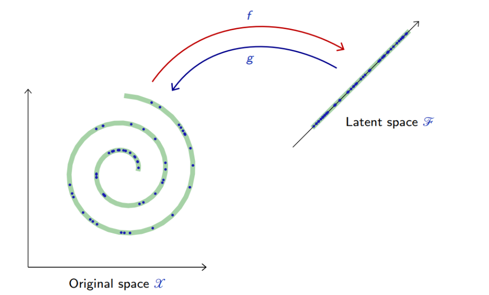
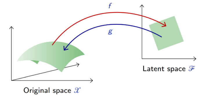
• Many applications such as image synthesis, denoising, super-resolution, speech synthesis or compression, require to go beyond classification and regression and model explicitly a high-dimensional signal.
• This modeling consists of finding “meaningful degrees of freedom”, or “factors of variations”, that describe the signal and are of lesser dimension.
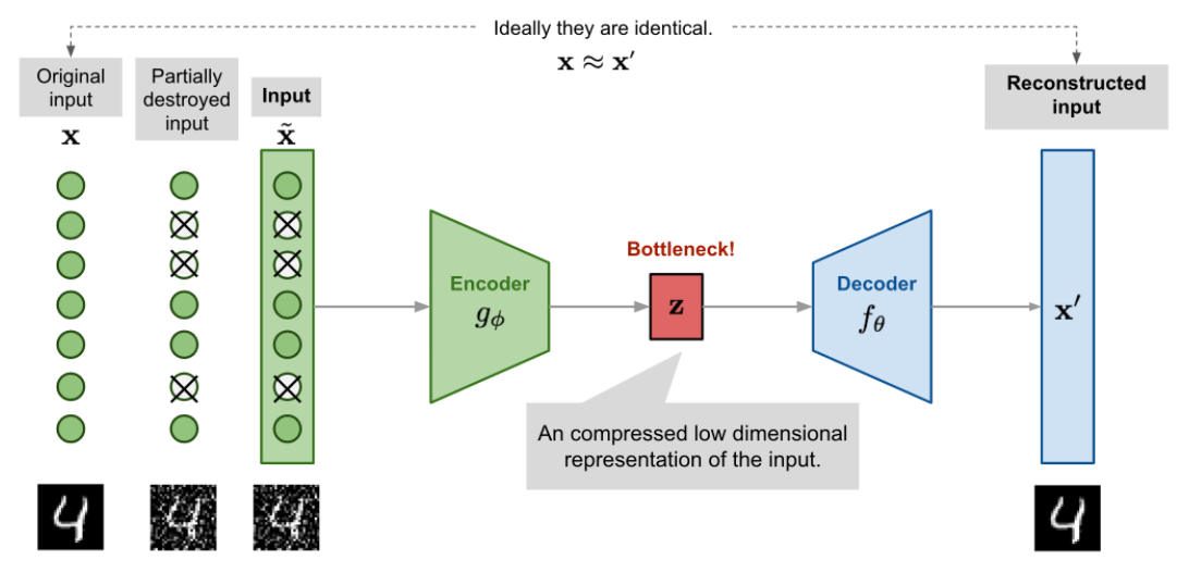
• Autoencoders are an unsupervised learning technique in which we leverage neural networks for the task of representation learning. Specifically, we’ll design a neural network architecture such that we impose a bottleneck in the network which forces a compressed knowledge representation of the original input.

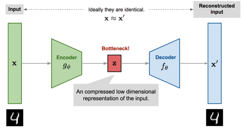
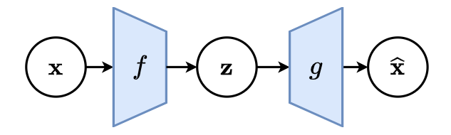
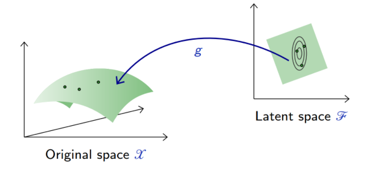
Mathematically, an Autoencoder is a composite function made of

• an encoder from the original space to a latent space ,
• a decoder to map back to ,

such that is close to the identity on the data.

Let be the data distribution over . A good auto-encoder could be characterized with the reconstruction loss

Given two parameterized mappings training consists of minimizing an empirical estimate of that loss

For example, when the auto-encoder is linear,

with the reconstruction error reduces to

In this case, an optimal solution is given by PCA.
Deep auto-encoders

Better results can be achieved with more sophisticated classes of mappings than linear projections: use deep neural networks for and .
For instance,

• by combining a multi-layer perceptron encoder with a multi-layer perceptron decoder
• by combining a convolutional network encoder with a decoder composed of the reciprocal transposed convolutional layers.

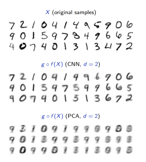
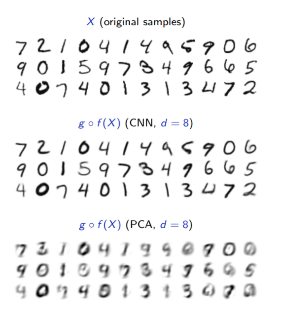
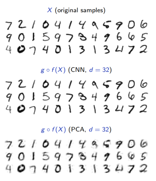
Compare Autoencoder with PCA on MNIST dataset

Denoising Autoencoder
Since the autoencoder learns the identity function, we are facing the risk of “overfitting” when there are more network parameters than the number of data points.
To avoid overfitting and improve the robustness, Denoising Autoencoder (Vincent et al. 2008) proposed a modification to the basic autoencoder. The input is partially corrupted by adding noises to or masking some values of the input vector in a stochastic manner, . Then the model is trained to recover the original input (note: not the corrupt one).

where defines the mapping from the true data samples to the noisy or corrupted ones.
Sampling from an AE’s latent space
The generative capability of the decoder in an auto-encoder can be assessed by introducing a (simple) density model over the latent space , sample there, and map the samples into the data space with .

For instance, a factored Gaussian model with diagonal covariance matrix,

where both are estimated on training data.

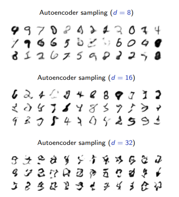
These results are not satisfactory because the density model on the latent space is too simple and inadequate.
Building a good model in latent space amounts to our original problem of modeling an empirical distribution, although it may now be in a lower dimension space.

II. Variational Inference

Latent variable model

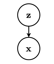
Consider for now a prescribed latent variable model that relates a set of observable variables to a set of unobserved variables .

The probabilistic model defines a joint probability distribution , which decomposes as

For a given model , inference consists in computing the posterior

For most interesting cases, this is usually intractable since it requires evaluating the evidence
: Intractable!

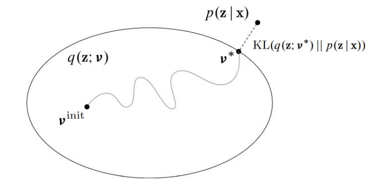
Variational inference turns posterior inference into an optimization problem.

• Consider a family of distributions that approximate the posterior , where the variational parameters index the family of distributions.
• The parameters are fit to minimize the KL divergence between the approximation and the posterior .
  Formally, we want to solve

For the same reason as before, the KL divergence cannot be directly minimized because of the term.
However, we can write

where is called the evidence lower bound objective.

• Since does not depend on , it can be considered as a constant, and minimizing the KL divergence is equivalent to maximizing the evidence lower bound, while being computationally tractable.
• Given a dataset , the final objective is the sum

Remark that

Therefore, maximizing the ELBO:

• encourages distributions to place their mass on configurations of latent variables that explain the observed data (first term);
• encourages distributions close to the prior (second term).
  Optimization
  We want
  
  We can proceed by gradient ascent, provided we can evaluate .

Evidence Lower Bound (ELBO)

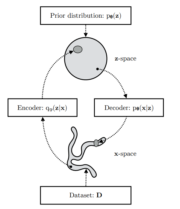
• A VAE learns stochastic mappings between an observed -space, whose empirical distribution is typically complicated, and a latent -space, whose distribution can be relatively simple (such as spherical).
• The generative model learns a joint distribution that is often (but not always) factorized as , with a prior distribution over latent space , and a schotastic decoder . The schochastic encoder also called inference model, approximates the true but intractable posterior of the generative model.

The second term is the Kullback-Leibler (KL) divergence between and , which is non-negative:

and zero if, and only if, equals the true posterior distribution.

The first term is the variational lower bound, also called the evidence lower bound (ELBO):

Due to the non-negativity of the KL divergence, the ELBO is a lower bound on the log-likelihood of the data.

So, interestingly, the KL divergence determines two ’distances’:

• By definition, the KL divergence of the approximate posterior from the true posterior;
• The gap between the ELBO and the marginal likelihood ; this is also called the tightness of the bound. The better approximates the true (posterior) distribution , in terms of the KL divergence, the smaller the gap.
  
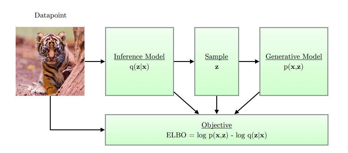
  Figure: Simple schematic of computational flow in a variational autoencoder.

Two for One
it can be understood that maximization of the ELBO w.r.t the parameters , will concurrently optimize the two things we care about:

• It will approximately maximize the marginal likelihood . This means that our generative model will become better.
• It will minimize the KL divergence of the approximation from the true posterior , so becomes better.

II. Variational Autoencoders

A variational auto-encoder is a deep latent variable model where:

• The prior is prescribed, and usually chosen to be Gaussian.

• The likelihood is parameterized with a generative network (or decoder) that takes as input and outputs parameters to the data distribution.
  

• The approximate posterior is parameterized with an inference network (or encoder) that takes as input and outputs parameters to the approximate posterior.
  

Stochastic Gradient-Based Optimization of the ELBO

As before, we can use variational inference, but to jointly optimize the generative and the inference networks parameters and .
We want

Given a dataset with i.i.d. data, the ELBO objective is the sum (or average) of individual-datapoint ELBO’s:

The individual-datapoint ELBO, and its gradient is, in general, intractable. However, good unbiased estimators exist, as we will show, such that we can still perform minibatch SGD.

Unbiased gradients of the ELBO w.r.t. the generative model parameters are simple to obtain:

Unbiased gradients w.r.t. the variational parameters are more difficult to obtain, since the ELBO’s expectation is taken w.r.t. the distribution , which is a function of . I.e., in general:

In the case of continuous latent variables, we can use a reparameterization trick for computing unbiased estimates of , as we will now discuss.

Reparameterization Trick
For continuous latent variables and a differentiable encoder and generative model, the ELBO can be straightforwardly differentiated w.r.t. both and through a change of variables, also called the reparameterization trick.

Change of variables

First, we express the random variable as some differentiable (and invertible) transformation of another random variable , given and :

where the distribution of random variable is independent of or .

Gradient of expectation under change of variable
Given such a change of variable, expectations can be rewritten in terms of

where and the expectation and gradient operators become commutative, and we can form a simple Monte Carlo estimator:

where in the last line, with random noise sample .

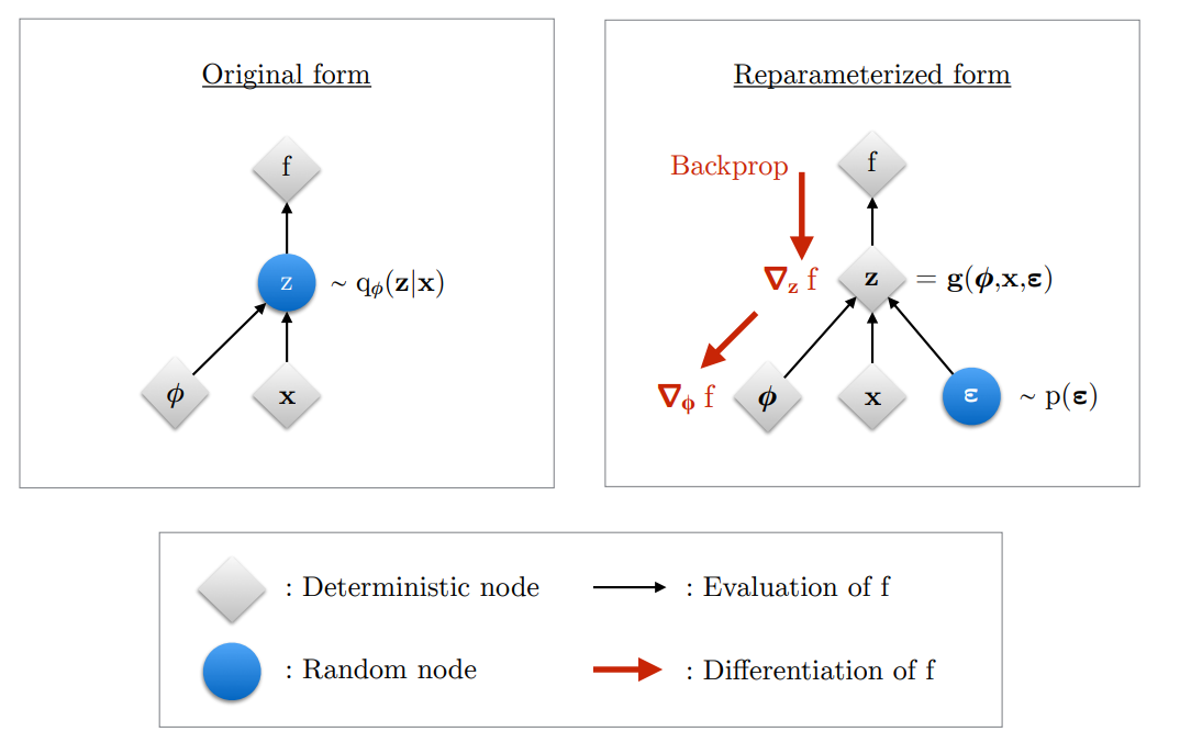
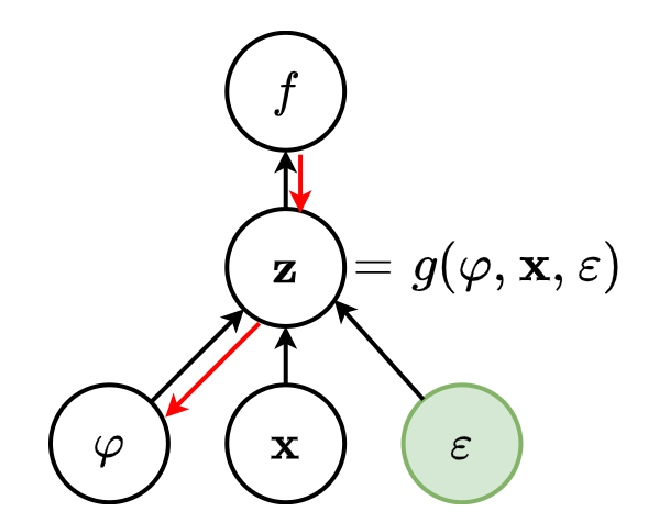
Figure: Illustration of the reparameterization trick. The variational parameters affect the objective through the random variable . We wish to compute gradients to optimize the objective with SGD. In the original form (left), we cannot differentiate w.r.t. , because we cannot directly backpropagate gradients through the random variable . We can “externalize” the randomness in by re-parameterizing the variable as a deterministic and differentiable function of , , and a newly introduced random variable . This allows us to “backprop through ”, and compute gradients .

For example, if , where and are the outputs of the inference network , then a common reparameterization is:

Given such a change of variable, the ELBO can be rewritten as:

Therefore,

which we can now estimate with Monte Carlo integration.

The last required ingredient is the evaluation of the likelihood given the change of variable . As long as is invertible, we have:

The Jacobian matrix contains all first derivatives of the transformation from to :

Example
Consider the following setup:

• Generative model:

• Inference model

Note that there is no restriction on the generative and inference network architectures. They could as well be arbitrarily complex convolutional networks.

Plugging everything together, the objective can be expressed as:

where the KL divergence can be expressed analytically as

which allows to evaluate its derivative without approximation.

III. Sample Python implementation

# Base Variational Autoencoder 
from torch import nn
from abc import abstractmethod

class BaseVAE(nn.Module):
    
    def __init__(self) -> None:
        super(BaseVAE, self).__init__()

    def encode(self, input: Tensor) -> List[Tensor]:
        raise NotImplementedError

    def decode(self, input: Tensor) -> Any:
        raise NotImplementedError

    def sample(self, batch_size:int, current_device: int, **kwargs) -> Tensor:
        raise NotImplementedError

    def generate(self, x: Tensor, **kwargs) -> Tensor:
        raise NotImplementedError

    @abstractmethod
    def forward(self, *inputs: Tensor) -> Tensor:
        pass

    @abstractmethod
    def loss_function(self, *inputs: Any, **kwargs) -> Tensor:
        pass

class VanillaVAE(BaseVAE):


    def __init__(self,
                 in_channels: int,
                 latent_dim: int,
                 hidden_dims: List = None,
                 **kwargs) -> None:
        super(VanillaVAE, self).__init__()

        self.latent_dim = latent_dim

        modules = []
        if hidden_dims is None:
            hidden_dims = [32, 64, 128, 256, 512]

        # Build Encoder
        for h_dim in hidden_dims:
            modules.append(
                nn.Sequential(
                    nn.Conv2d(in_channels, out_channels=h_dim,
                              kernel_size= 3, stride= 2, padding  = 1),
                    nn.BatchNorm2d(h_dim),
                    nn.LeakyReLU())
            )
            in_channels = h_dim

        self.encoder = nn.Sequential(*modules)
        self.fc_mu = nn.Linear(hidden_dims[-1]*4, latent_dim)
        self.fc_var = nn.Linear(hidden_dims[-1]*4, latent_dim)


        # Build Decoder
        modules = []

        self.decoder_input = nn.Linear(latent_dim, hidden_dims[-1] * 4)

        hidden_dims.reverse()

        for i in range(len(hidden_dims) - 1):
            modules.append(
                nn.Sequential(
                    nn.ConvTranspose2d(hidden_dims[i],
                                       hidden_dims[i + 1],
                                       kernel_size=3,
                                       stride = 2,
                                       padding=1,
                                       output_padding=1),
                    nn.BatchNorm2d(hidden_dims[i + 1]),
                    nn.LeakyReLU())
            )



        self.decoder = nn.Sequential(*modules)

        self.final_layer = nn.Sequential(
                            nn.ConvTranspose2d(hidden_dims[-1],
                                               hidden_dims[-1],
                                               kernel_size=3,
                                               stride=2,
                                               padding=1,
                                               output_padding=1),
                            nn.BatchNorm2d(hidden_dims[-1]),
                            nn.LeakyReLU(),
                            nn.Conv2d(hidden_dims[-1], out_channels= 3,
                                      kernel_size= 3, padding= 1),
                            nn.Tanh())

    def encode(self, input: Tensor) -> List[Tensor]:
        """
        Encodes the input by passing through the encoder network
        and returns the latent codes.
        :param input: (Tensor) Input tensor to encoder [N x C x H x W]
        :return: (Tensor) List of latent codes
        """
        result = self.encoder(input)
        result = torch.flatten(result, start_dim=1)

        # Split the result into mu and var components
        # of the latent Gaussian distribution
        mu = self.fc_mu(result)
        log_var = self.fc_var(result)

        return [mu, log_var]

    def decode(self, z: Tensor) -> Tensor:
        """
        Maps the given latent codes
        onto the image space.
        :param z: (Tensor) [B x D]
        :return: (Tensor) [B x C x H x W]
        """
        result = self.decoder_input(z)
        result = result.view(-1, 512, 2, 2)
        result = self.decoder(result)
        result = self.final_layer(result)
        return result

    def reparameterize(self, mu: Tensor, logvar: Tensor) -> Tensor:
        """
        Reparameterization trick to sample from N(mu, var) from
        N(0,1).
        :param mu: (Tensor) Mean of the latent Gaussian [B x D]
        :param logvar: (Tensor) Standard deviation of the latent Gaussian [B x D]
        :return: (Tensor) [B x D]
        """
        std = torch.exp(0.5 * logvar)
        eps = torch.randn_like(std)
        return eps * std + mu

    def forward(self, input: Tensor, **kwargs) -> List[Tensor]:
        mu, log_var = self.encode(input)
        z = self.reparameterize(mu, log_var)
        return  [self.decode(z), input, mu, log_var]

    def loss_function(self,
                      *args,
                      **kwargs) -> dict:
        """
        Computes the VAE loss function.
        KL(N(\mu, \sigma), N(0, 1)) = \log \frac{1}{\sigma} + \frac{\sigma^2 + \mu^2}{2} - \frac{1}{2}
        :param args:
        :param kwargs:
        :return:
        """
        recons = args[0]
        input = args[1]
        mu = args[2]
        log_var = args[3]

        kld_weight = kwargs['M_N'] # Account for the minibatch samples from the dataset
        recons_loss =F.mse_loss(recons, input)


        kld_loss = torch.mean(-0.5 * torch.sum(1 + log_var - mu ** 2 - log_var.exp(), dim = 1), dim = 0)

        loss = recons_loss + kld_weight * kld_loss
        return {'loss': loss, 'Reconstruction_Loss':recons_loss.detach(), 'KLD':-kld_loss.detach()}

    def sample(self,
               num_samples:int,
               current_device: int, **kwargs) -> Tensor:
        """
        Samples from the latent space and return the corresponding
        image space map.
        :param num_samples: (Int) Number of samples
        :param current_device: (Int) Device to run the model
        :return: (Tensor)
        """
        z = torch.randn(num_samples,
                        self.latent_dim)

        z = z.to(current_device)

        samples = self.decode(z)
        return samples

    def generate(self, x: Tensor, **kwargs) -> Tensor:
        """
        Given an input image x, returns the reconstructed image
        :param x: (Tensor) [B x C x H x W]
        :return: (Tensor) [B x C x H x W]
        """

        return self.forward(x)[0]

IV. References

1. From Autoencoder to Beta-VAE,
   https://lilianweng.github.io/posts/2018-08-12-vae/?fbclid=IwAR3-2GNNEw1dv7oHshWhMfB9F9wym4nMHtu1VZc1pOvlC1Qq_ZBOXN2H0ag

2. Diederik P. Kingma, Max Welling, An Introduction to Variational Autoencoders

3. Diederik P Kingma, Max Welling, Auto-Encoding Variational Bayes, ICLR 2014

4. Lecture 10: Auto-encoders and variational auto-encoders, https://github.com/glouppe/info8010-deep-learning